The present simulation project continues the earlier project P1 by working out the generalization to more than one particles, to which only a short remark was made in P1. As in P1 we start with a single particle with a wave function concentrated on only a part of its finite discrete configuration space. Notions and methods will be taken from P1. Among them there is the notion of a biotope of a particle, which, without explanation may be considered strange. Beside the spatial concentration, our initial wave function is prepared to show a group velocity (to the right). Time evolution as implemented by a numerical integrator will make the wave function eventually reach the right rim of the biotope (in the sense of having non-vanishing values there). Due to the tendency of concentrated wave functions to broaden, it will sometime also reach the left rim. In order to continue with the time evolution without disturbation we have to extend the biotope on the side of 'contact'. If this is the left end we simply attach a copy of the original biotope. In case of the right boundary we attache a modified copy of the original biotope: one that hosts at its center a bound particle, held by the potential well of an external force field of finite reach. Of course we assume the new particle to be in its ground state. Then the new wave function is the tensor product of the old wave function and the known ground state wave function. Of course, the total number of particles grew by 1. In the course of time we will have many particles and many potential wells. Then the interactions to be included into the many-particle Hamiltonian are as in a hypothetical electrostatics of finite range in which all particles carry the same charge and all potential wells originate from opposite charges fixed in space. The repulsive interaction of particles implied by this picture is also part of our model. All interaction potentials have the same finite reach and all particle-particle interactions are the same as functions of distance. The same holds for all particle-well potentials. Finally we set up things such that all bound particles are in the ground state when coming into existence, and that biotope extension according to the given rules becomes effective if the many-particle wave function touches the rim of the biotope. A computable criterion for this is obvious.
We have now set the stage for a process in which a single particle runs into a highly idealized crystal and, in doing so, comes into contact and interaction with more and more particles. In the present project we stop our simulation of the process at the point where we had to add a fourth particle and thus would slow down execution to an intolerable level.
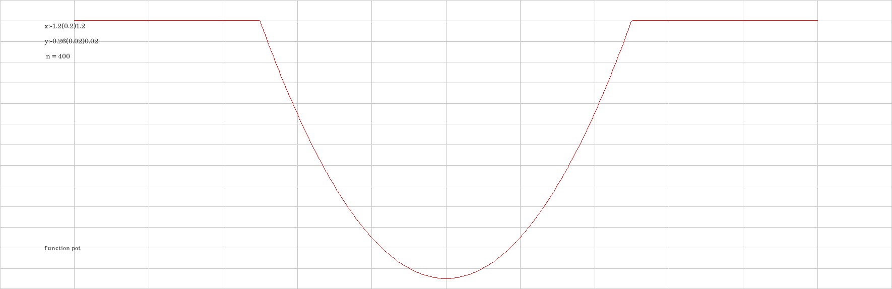
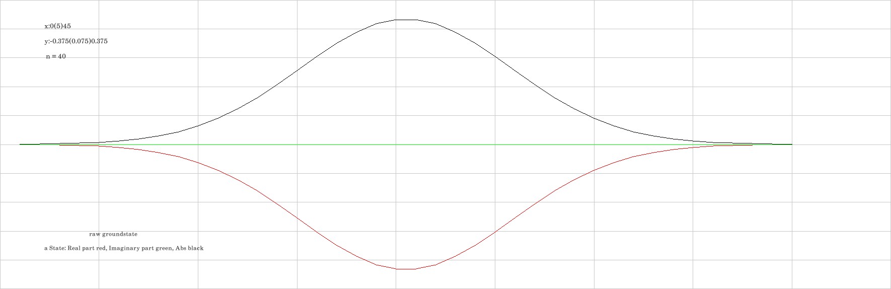
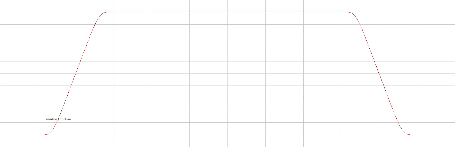
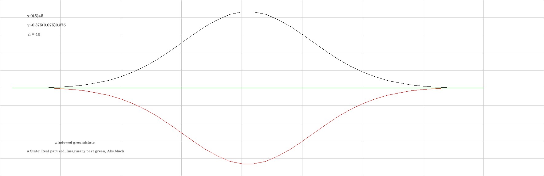
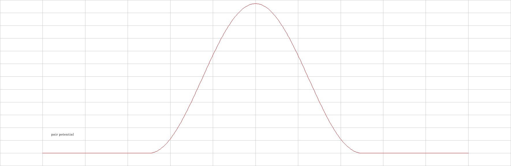
Now we have to define the objects introduced so far only in broad outline. To support this endeavor is the task of the first of the present two videos. The first part of this video consists of a few 'still images', each being a sequence of five identical images. Using a viewer program like the VLC media player one is able to stop the video in a way that one is able to inspect each of them. Even more convenient is to use the links, the first one being img1. This shows a parabolic potential well (named pot in the diagram) at the center of the original biotope. The width of the well, its depth, the number discrete positions in the biotope, and the mass of a particle are arranged such that the wave function of the ground state approximately vanishes at the rim of the biotope. Assuming that the particle is in its ground state initially it will stay within its biotope, unless interaction with nearby particles changes its initially stationary state into a non-stationary one. If one would require that the wave function of the bound state has very low values on the boundary of the biotope one would need so many discrete positions in the biotope that time evolution becomes quite expensive to compute. A good compromise is chosen in the present simulation with 40 points (corresponding to a 40-dimensional state space). The ground state, as obtained with a numerical method from the Eigen3-library is shown here. Perfect vanishing at the boundary turns out to be necessary if disturbing artifacts during time evolution are to be avoided. So we muliply the state with a window function and get this function. The window function is a numerical version of a smooth mathematical function. Details are here. The newly attached particles do not only feel forces from the potential wells, but also from the companion particles. Here this interaction is assumed to be repulsive and of finite range. The interaction potential is given by the following graphics. the we start with a simple system, an idealized non-relativistic free quantum particle moving in a finite 1-dimensional discrete space. The initial wave function is given such that the step-wise time evolution algorithm allows at least a few steps before the the wave function no longer vanishes on one of the two boundary points of its biotope. xxx As in this simulation project we consider the dynamics of a non-relativistic particle moving in a finite 1-dimensional discrete space. The initial wave function is similar to the discrete version of a Gaussian wave packet moving with constant velocity to the right. When the particle has reached the right rim of its available space (its biotope as I call it) the biotope will be enlarged by attaching a modified copy of the original biotope to it. The modification consists of a bound particle in its ground state which sits at the center of the attached biotope. If the moving wave packet, due to its broadening trend, happens to reach the left rim of the biotope we also attach a copy of the original biotope to it --- this time without modification, i. e. without adding a particle. This sets the stage for a process in which a single particle runs into a highly idealized crystal and, in doing so, comes into contact and interaction with more and more particles. In the present project we stop our simulation of the process at the point where we had to add a fourth particle and thus would slow down execution to an intolerable level.
Now we have to define the objects introduced so far only in broad outline. To support this endeavor is the task of the first of the present two videos. The first part of this video consists of a few 'still images', each being a sequence of five identical images. Using a viewer program like the VLC media player one is able to stop the video in a way that one is able to inspect each of them. Even more convenient is to use the links, the first one being img1. This shows a parabolic potential well (named pot in the diagram) at the center of the original biotope. The width of the well, its depth, the number discrete positions in the biotope, and the mass of a particle are arranged such that the wave function of the ground state approximately vanishes at the rim of the biotope. Assuming that the particle is in its ground state initially it will stay within its biotope, unless interaction with nearby particles changes its initially stationary state into a non-stationary one. If one would require that the wave function of the bound state has very low values on the boundary of the biotope one would need so many discrete positions in the biotope that time evolution becomes quite expensive to compute. A good compromise is chosen in the present simulation with 40 points (corresponding to a 40-dimensional state space). The ground state, as obtained with a numerical method from the Eigen3-library is shown here. Perfect vanishing at the boundary turns out to be necessary if disturbing artifacts during time evolution are to be avoided. So we muliply the state with a window function and get this function. The window function is a numerical version of a smooth mathematical function. Details are here. The newly attached particles do not only feel forces from the potential wells, but also from the companion particles. Here this interaction is assumed to be repulsive and of finite range. The interaction potential is given by the following graphics.
In the present simulation, the particle we have been speaking about so far, will appear in two roles:
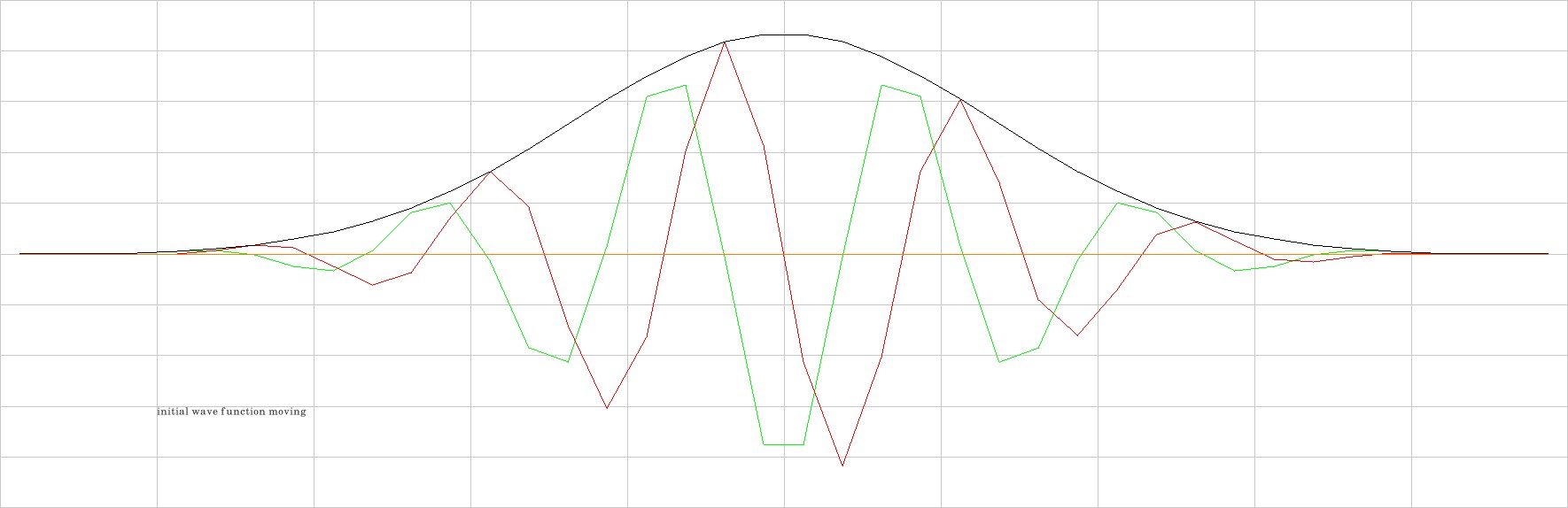
1. Its wave function, after given a uniform speed (to the right) by a kinematical boost transformation, will be taken as the initial state of our system (one free particle, no potential well in its biotope). This wave function is shown here. The edgy nature of the curves representing real and imaginary part of the wave function show that a finer discretization of position would be convenient.
2. Without boost transformation and with the potential well we have the system which will be appended to the right if any of the particles touches the right boundary of the biotope.
Both videos show how the system grows up to three particles. The tog files cpmcerr...txt in the directories ./r230321a and ./r230323a show that for three particles the execution of the time evolution is achingly slow.
It should be noted that for more than 1 particle the graphics don't show the wave function but a useful derived quantity: the probability to find a particle in a place if the positions of all other particles were determined simultaneously. This gives a curve for each particle with different colors corresponding to different particles.
These computing tools were used: CPU 4.464 GHz; RAM 16 GB; OS Ubuntu; SW C++20, OpenGL, FreeGlut, Eigen3, Code::Blocks, ffmpeg (for video creation from ppm-files), ImageMagick (for conversion from ppm to jpg), C+- (self-made C++ library); Compiler GNU.